You open a micrograph, outline an object in ImageJ, and the Results table immediately shows "452.39". Two questions follow: in what unit, and why should you believe it?
Many tutorials stop at "click Measure", but the steps before that click decide the result. This guide uses a simulated image drawn by a macro, so the true sizes are known, and deliberately gets calibration, thresholding and resizing wrong to see how far the numbers move.
Bottom line: software producing a number does not mean the measurement method has been validated. Every number here comes from a simulated image and illustrates the method. None is a metrologically calibrated measurement.
Environment (2026-11-09): ImageJ 1.54g (Ubuntu package) on Linux, run as a batch macro. Menu paths follow the official documentation and have not yet been walked through in the Fiji interface.
1. A pixel is not a length
An uncalibrated image only knows how many pixels something covers. Change the objective and the same object covers a different number of pixels, so pixel values cannot be compared directly across images.
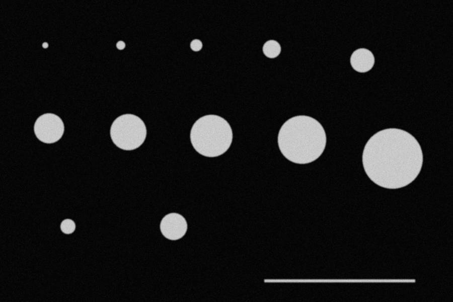
To get physical size you need the length of one pixel. In the demo image a 400-pixel scale bar represents 100 µm:
1 pixel = 100 µm / 400 = 0.25 µm
area factor = 0.25² = 0.0625 µm² per pixel
Area scales with the square of the calibration, which matters in the failures below.
2. Make a practice image you can reproduce
In Fiji, choose Plugins > New > Macro, paste this macro, change the first line to your output folder and click Run.
out = "/path/to/your/folder/";   // keep the final slash; use / on Windows too
newImage("demo", "8-bit black", 1200, 800, 1);
setColor(200);
fillOval(340 - 48, 350 - 48, 96, 96);     // diameter 96 px = 24 µm
fillOval(320 - 12, 120 - 12, 24, 24);     // diameter 24 px = 6 µm
fillRect(700, 740, 400, 8);               // 400 px scale bar = 100 µm
run("Select None");
run("Gaussian Blur...", "sigma=1.5");     // simulates optical blur
random("seed", 42);
run("Add Specified Noise...", "standard=8");
run("Set Scale...", "distance=400 known=100 unit=um");
run("Set Measurements...", "area perimeter feret's display redirect=None decimal=4");
setAutoThreshold("Otsu dark");
run("Analyze Particles...", "size=20-Infinity pixel circularity=0.70-1.00 show=Nothing display exclude clear");
saveAs("Results", out + "results.csv");
The macro runs the whole chain: create the image, calibrate, choose measurements, threshold, extract objects and export a table. On ImageJ 1.54g it outputs areas of 27.75 µm² (6 µm circle) and 452.63 µm² (24 µm circle), which you can use to check your setup. The scale bar is long and thin, so circularity=0.70-1.00 excludes it.
The full experiment script is imagej_measurement_demo.ijm. Its image has 12 circles from 16 to 160 pixels across.
3. The same steps by hand
Before relying on macros, walk through the menus once:
- Calibrate: draw a line along the scale bar with the straight-line tool, open Analyze > Set Scale, and enter 100 for Known distance and um for Unit. Leave Global unticked unless every image has the same magnification.
- Choose measurements: in Analyze > Set Measurements, tick Area, Perimeter, Feret's diameter and so on. This sets the columns produced by Measure and Analyze Particles.
- Measure by hand: draw an ROI with the line, oval or polygon tool and press M (Analyze > Measure). ROIs can be saved in the ROI Manager so that someone else can check them.
- Threshold: in Image > Adjust > Threshold, choose a method and record the limits.
- Extract in bulk: in Analyze > Analyze Particles, set the size and circularity ranges.
- Export: in the Results window, use File > Save As to save a CSV.
4. Reference result
With the Otsu automatic threshold (lower limit 101 for this image), areas were:
| True diameter | True area (µm²) | Measured area (µm²) | Relative error |
|---|---|---|---|
| 4 µm (16 px) | 12.57 | 12.81 | +1.96% |
| 6 µm (24 px) | 28.27 | 27.69 | −2.08% |
| 12 µm (48 px) | 113.10 | 112.25 | −0.75% |
| 24 µm (96 px) | 452.39 | 451.50 | −0.20% |
| 40 µm (160 px) | 1256.64 | 1256.31 | −0.03% |
The pattern is clear: the fewer pixels an object covers, the larger the relative error.
One more detail. Feret's diameter is the longest distance between any two points on the selection boundary. For the 24 µm circle, Feret was 24.31 µm, 1.3% above the true value, while MinFeret was exactly 24.00 µm. A pixelated circle is not an ideal circle, so when you report a "diameter", say whether it is Feret, MinFeret or the equivalent diameter from area.
5. Four deliberate mistakes
Threshold
Same image, different lower limit:
| Lower limit | Area error, 24 µm circle | Area error, 6 µm circle |
|---|---|---|
| 60 | +3.35% | +10.30% |
| 100 | −0.18% | −1.63% |
| 140 | −3.54% | −15.34% |
| 180 | −8.91% | −33.24% |
Image edges are gradual, and the threshold decides where the boundary is. It is not a display setting but part of the definition of the measurement. State it in your methods and keep it constant within a batch.
Wrong calibration value
Enter the scale bar as 110 µm by mistake and lengths grow by 10% and areas by about 21% (1.1² = 1.21). The 24 µm circle goes from 451.50 to 546.32 µm², and the software gives no warning.
Resizing the image
After reducing the image to 50%:
- With Image > Scale inside ImageJ, the calibration is updated, the pixel width becomes 0.5 µm, and the largest circle is still 1257.75 µm².
- Apply the old calibration to the smaller image and the area becomes 314.44 µm², a quarter of the correct value.
This is a common real-world error: an image is resized in PowerPoint or a screenshot tool, and the old calibration is reused. Measure original files, such as the TIFF exported by the microscope, whenever possible.
Changing magnification
Change the objective or camera settings and the length per pixel changes, so the old calibration no longer applies. The Global option in Set Scale applies one scale to images opened later, which invites mistakes when magnifications are mixed.
6. Good repeatability is not accuracy
Changing the noise seed 10 times and measuring the same 24 µm circle with Otsu and with a fixed threshold of 170 gave:
| Method | Mean area of 10 runs | SD | Bias from true value |
|---|---|---|---|
| Otsu | 451.63 µm² | 0.22 | −0.17% |
| Fixed threshold 170 | 422.62 µm² | 0.37 | −6.58% |
The fixed threshold results are tightly grouped, with a coefficient of variation of just 0.087%, yet consistently 6.58% too small. That is the difference between repeatability (results agree with each other) and trueness (results agree with the true value). Reporting only that repeated measurements agree says nothing about whether they are right.
Only the synthetic noise changed here. There was no new specimen, focusing, imaging or operator, so this SD is far smaller than real experimental repeatability and is not a performance figure for any real method.
Re-running the macro with the same seed produced two identical CSV files. That shows only that the calculation is reproducible.
7. Edges, and what this image does not cover
The simulated objects are clear and separate on an even background. Real images bring touching objects, uneven illumination, defocus, objects with no well-defined edge, and lens distortion. Then a threshold plus Analyze Particles is often not enough: you may need preprocessing, watershed splitting or manual review, and you must check the bias those steps introduce.
8. What papers or inspection work also require
- Calibrate under the same conditions against a traceable standard, such as a stage micrometer, rather than the scale bar in the image.
- Estimate bias using specimens of known size.
- Assess real repeatability and reproducibility with new specimens, new images and different operators.
- Record the software version, algorithm, threshold and parameters, and keep the macro and ROIs.
For uncertainty evaluation and method agreement, continue with Errors and validation in scientific image measurement.
9. Who this is for
Suitable for: researchers and students measuring area, length or particle counts, especially those who want to turn manual steps into a checkable macro.
Do not apply as is to: work that must produce metrological or inspection conclusions, or images with heavy overlap that need deep-learning segmentation. The first needs validation under the relevant standard, and the second may need dedicated tools.